In this post I aim to visually, mathematically and programatically explain the gradient, and how its understanding is crucial for gradient descent. For those unfamiliar, gradient descent is used in various ML models spanning from logistic regression, to neural nets. Ultimately, gradient descent, and transitively the gradient, are the blueprints that guide these models to converge on ideal weights.
In short, The gradient is an n-dimensional generalization of the derivative, which can be applied in any direction.
For a complete understanding of the content in this post, I would suggest a firm understanding of the following topics:
- Derivatives and the Chain Rule (Calculus)
- Partial Derivatives (Multivariate Calculus)
- Basic Vector Operations (Linear Algebra)
- Objective Functions (Also called Loss Function)
- Basic Understanding of NumPy
The Data
Our dataset is made up of South Boston home sales, and consists of 2 very simple column vectors:
The Model
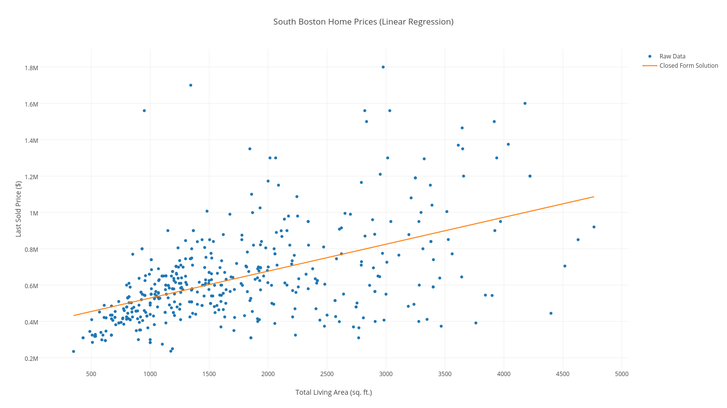
We will be learning a simple Linear Regression model, that predicts a home in South Boston’s value (sale price) based solely on the Living Area of the property. We want to fit a line to our data, defined by:
Our line should overlay our data as follows:
 Thus, our main objective is to minimize the distance between each point and our line. We will use Mean Squared Error as our objective function, which is a fancy way of saying: “For each point (x, y) in our dataset, take the squared distance between the y-value, and the predicted y-value, and add them all up. Then divide by the number of examples, n.”
In mathematical fancy notation, the Mean Squared Error looks as follows:
Using our above objective function, (\(y_{i,predicted} = ax_{i} + b,\)) we get:
Our goal is to minimize this function, and we do so with the gradient.
Let’s begin with the most naive solution to find our minimum: take every combination of \(a\) and \(b\), then find the combination that yields the lowest error \(J(a, b\)).
The problem: What if (rather than \(a\) and \(b\) ) we have 10,000 variables to solve for? We would find ourselves in a permutational nightmare that no computer could handle!
We need a way to gracefully and quickly find our minimum: and we use the gradient to do so.
The Math: Finding the Gradient
The gradient is a vector of the partial derivatives of a function. It is the n-dimensional generalization of the derivative, defining the rate of change with respect to all “n” variables. It is usually written as follows:
In our case, we need to find both partial derivatives of \(J(a, b)\) - we use the Chain Rule to do so:
Don’t be intimidated by the summation notion when calculating the partials! We are just differentiating the function to the right of the symbol!
Rearranging terms, and distributing terms we get our gradient:
The Math: Visualizing the Gradient’s Significance
If we are standing on the mountain-like curve of our objective function, at point \((a, b)\), we want to find the direction with the greatest rate of negative change.
In other words, we want to find the steepest path down the mountain, because the lower our error (height of our curve), the more accurate our model! Below is the surface of our objective function \(J(a, b)\), and our starting point \((a=340, b=380000)\):
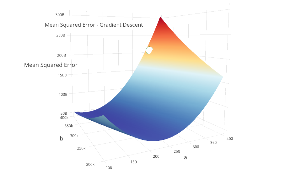
Which direction do we step? It turns out that the direction of the gradient vector, at a given point, will naturally point in the steepest direction!
The gradient will be our guide down the mountain!
The Math: Proving the Gradient’s Significance
Here’s where things get a bit “mathy”. Let’s prove why the direction of the gradient vector points in the direction of greatest change.
The rate-of-change of \(J(a, b)\), in a certain direction, \(\vec v\), with respect to distance traveled (\(ds\)), is defined as the gradient dotted with a vector indicating the direction to travel (\(\vec v)\), or:
All we are saying is that given an arbitrary direction, \(\vec v\), down our mountain, if we travel that direction in \(ds\) units, our error, \(J\), changes at a rate described by the above formula, which depends on the gradient.
Using the definition of the dot-product (\(x \cdot y = ||x||\ ||y||\ cos(\theta_{x,y})\)), we can re-write this as the product of each vector’s magnitude, times the cosine of the angle between them:
To maximize the rate of change, we would want to maximize \(cos(\theta)\) by setting \(\theta = 0\), to get \(1\), the highest possible value of the \(cos()\) function.
If the angle between these two vectors is \(0\), then the two vectors are parallel, therefore:
Our steepest step is in the direction of the gradient! So we want to travel in the opposite direction of the gradient, by multiplying it by \(-1\). If you take anything away from this post, remember this!
Given this fact, at each “step” along our descent, we:
- Calculate our gradient at the point \( (a, b) \).
-
We want the negative gradient, so we travel downhill and not uphill!
-
- Multiply the gradient by a scalar, (also called a learning rate, denoted by \(\eta\))
- The learning rate is what we call a hyperparameter, and can be tweaked to ensure convergence. Set too high or low, the model might converge!
- Update our weights using our multiplied gradient:
- Terminate if we have converged!
The Math: Implementing Gradient Descent
The equivalent code, implemented using Python and NumPy looks as follows:
import numpy as np
# I've experimented w/ Python3.6 unicode symbols in this snippet
def gradient_descent_mse(x_vec, y_vec):
    n = len(x_vec)
    # Define Partials & Objective Function (MSE)
    def J(a, b):
        return np.sum(((a * x_vec + b) - y_vec) ** 2 / n)
    def dJ_db(a, b):
       return np.sum((a * x_vec + b) - y_vec) / n
    def dJ_da(a, b):
       return np.sum(x_vec * ((a * x_vec + b) - y_vec)) / n
    # Initialize our weights
    a = 350
    b = 380000
    Δj = np.Infinity
    j = J(a, b)
    # Convergence Conditions
    δ = 1
    max_iterations = 150
    # Learning Rates (separate rate for each partial)
    ŋ_b = .15
    ŋ_a = .00000005
    i = 0
    while abs(Δj) > δ and i < max_iterations:
        i += 1
        # Find the gradient at the point (a, b)
        grad = [dJ_da(a, b), dJ_db(a, b)]
        # Multiply each partial deriv by its learning rate
        Δa = grad[0] * -ŋ_a
        Δb = grad[1] * -ŋ_b
        # Update our weights
        a += Δa
        b += Δb
        # Update the error at each iteration
        j_new = J(a, b)
        Δj = j - j_new
        j = j_new
    print("y = {0}x + {1}".format(str(a), str(b)))
We stop our descent when we have maxed out on iterations, or when we see (very small) decreases in the error calculated by \(J\).
To visualize our graceful descent, the following surface plots 150 iterations of our Gradient Descent, and shows us converging on \( a \approx 148, b \approx 380000\).
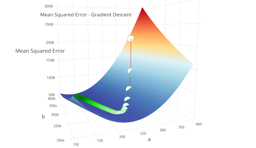
You can clearly see the “path down the mountain”, and visually grasp how the algorithm actually converges.
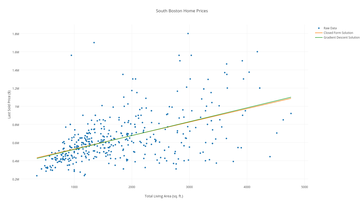
Our final “line of best fit” after 150 iterations, superimposed atop our data, and the closed-form solution, looks almost identical to our closed-form solution (if we had iterated 100 more times, the lines would have been superimposed, and indistinguishable!):
Conclusion
In our example here, we have mathematically, programatically, and visually proved the effectiveness of Gradient Descent in minimizing Objective Functions. Perhaps more importantly, we have shed light on the gradient, and why it is such a graceful solution to our error minimization.
There are many flavors of Gradient Descent, other than the (naive) implementation provided above. Stochastic Gradient Descent (SGD) is the most commonly used algorithm for minimizations, and is found everywhere from Logistic Regression Classifiers, to Deep Learning and Neural Nets.
Some of you may point out that the above example is trivial! There is a closed solution to this problem of Least Squares Regression! We’ve used this example for simplicity’s sake to introduce The Gradient and Gradient Descent. This post on solving Logistic Regression iteratively, addresses a more practical problem: there is no closed form solution to Logistic Regression!