We’ve explored gradient descent, but we haven’t talked about learning rates, and how these hyperparameters are the key differentiators between convergence, and divergence.
More specifically, let’s visually explore what happens when we set our learning rate to be too high, and talk about strategies to avoid divergence.
The Code
As a refresher, in our example we are trying to minimize the Mean Squared Error (MSE) with gradient descent, by choosing ideal values for (\(a, b\)). Details can be found in the previous post on the gradient
import numpy as np
# I've experimented w/ Python3.6 unicode symbols in this snippet
def gradient_descent_mse(x_vec, y_vec):
    n = len(x_vec)
    # Define Partials & Objective Function (MSE)
    def J(a, b):
       return np.sum(((a * x_vec + b) - y_vec) ** 2 / n)
    def dJ_db(a, b):
       return np.sum((a * x_vec + b) - y_vec) / n
    def dJ_da(a, b):
       return np.sum(x_vec * ((a * x_vec + b) - y_vec)) / n
    # Initialize our weights
    a = 250
    b = 250000
    Δj = np.Infinity
    j = J(a, b)
    # Convergence Conditions
    δ = 1
    max_iterations = 150
    # Learning Rates ()
    ŋ_b = .15
    ŋ_a = .00000005
    i = 0
    while abs(Δj) > δ and i < max_iterations:
        i += 1
        # Find the gradient at the point (a, b)
        grad = [dJ_da(a, b), dJ_db(a, b)]
        # Multiply each partial deriv by its learning rate
        Δa = grad[0] * -ŋ_a
        Δb = grad[1] * -ŋ_b
        # Update our weights
        a += Δa
        b += Δb
        # Update the error at each iteration
        j_new = J(a, b)
        Δj = j - j_new
        j = j_new
    print("y = {0}x + {1}".format(str(a), str(b)))
Plotting our Gradient Descent
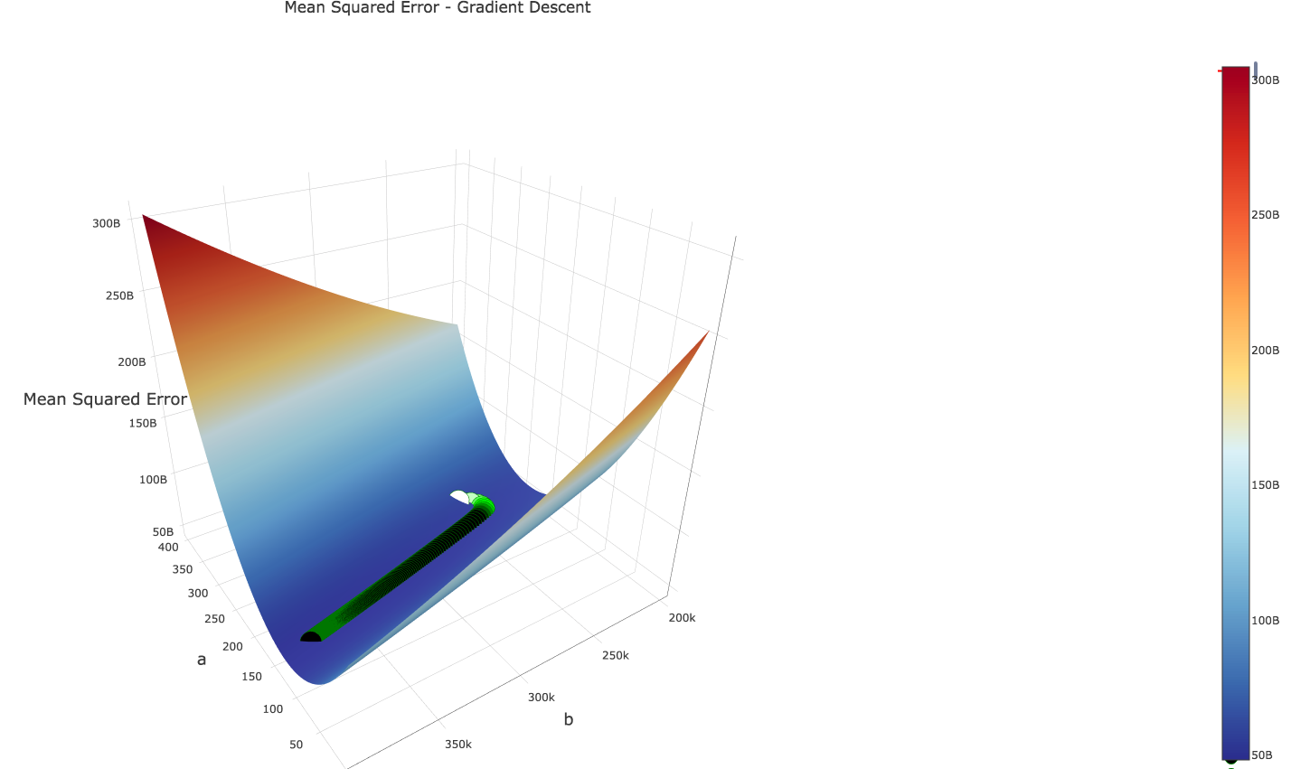
When we plot the iterations of our gradient descent algorithm with the above learning rates, we see that we are guided in the right direction by gradient descent:
Let’s now see what happens if we bump up the learning rate of our variable \(a\) by a factor of ~10…
    ŋ_b = .15
    #ŋ_a =.00000005
    ŋ_a = .000000575
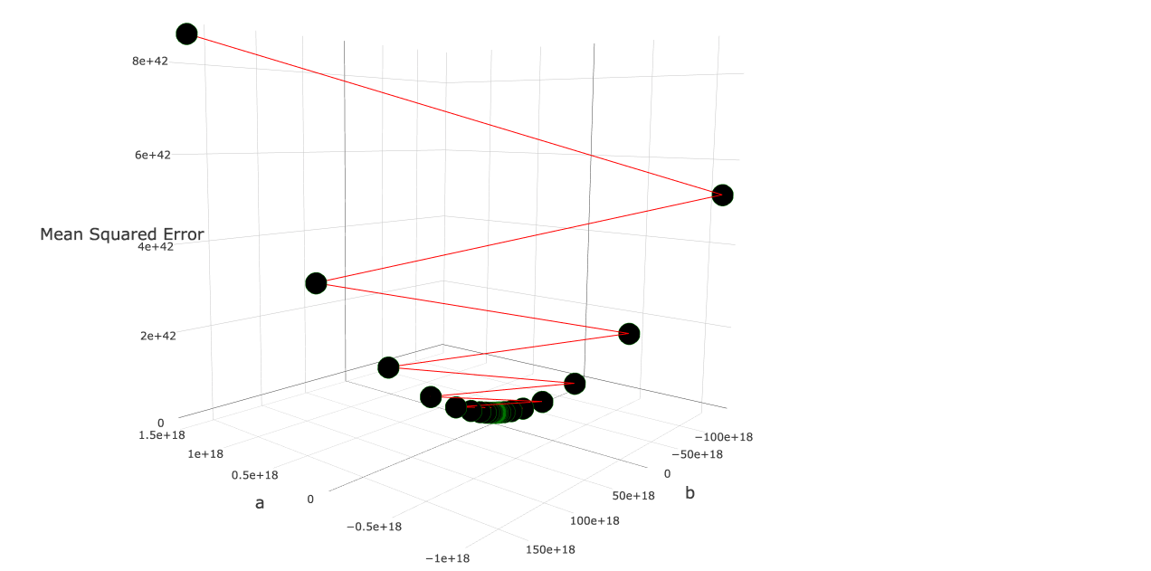
Huh? What happened here? Our z-axis has a range of \([0…8e+42]\); many magnitudes greater than our “good” graph, causing our “objective function surface” to disappear into oblivion. Additionally, our error is increasing with every iteration!
Let’s cut the number of iterations down from 150, to 7 to see what is actually going on:
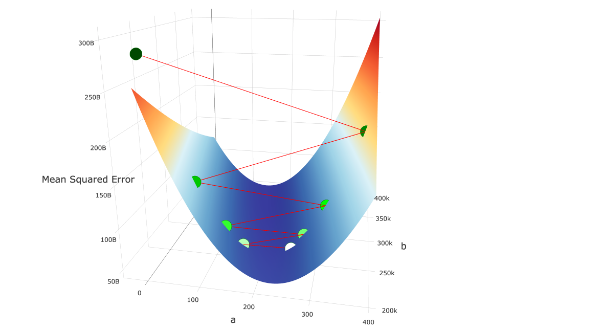
Ok. So that makes a bit more sense. Here’s what’s happening:
- We start at the white point in the “valley”, and calculate the gradient at that point.
- We multiply our learning rates by our gradient and move along this vector to our new point (the slightly greenish point to the left of the white point)
- Because our learning rate was so high, combined with the magnitude of the gradient, we “jumped over” our local minimum.
- We calculate our gradient at point 2, and make our next move, again, jumping over our local minimum
- Our gradient at point 2 is even greater than the gradient at point 1!
- Our next step will again, jump over our valley, and we will rinse and repeat for eternity…
- Due to the convex, valley-like curve of our objective function, as we continue to jump from side to side, the gradient at each jump grows higher. Our error increases quadratically with each “jump”, and our algorithm diverges to infinite error.
Note: Just the “valley-jumping” alone is a problem that needs fixing - it can lead to slow convergence, and worse, divergence. I’ve chosen this example with runaway quadratic ascension because it was an easy way to choose a diverging gradient descent.
Remedies
Of course, we can manually tweak our learning rates for each weight until we find that our model converges.
Or, naively, to prevent our “runaway gradient ascent”, we could implement a simple check for this case in our loop. If we gain error (rather than losing it), we can divide the deltas (which get added to our weights) by 2, until we see a drop in error. (Line 8 below)
    while abs(Δj) > δ and i < max_iterations:
        i += 1
        # Find the gradient at the point (a, b)
        grad = [dJ_da(a, b), dJ_db(a, b)]
        # Multiply each partial deriv by its learning rate
        Δa = grad[0] * -ŋ_a
        Δb = grad[1] * -ŋ_b
        while J(a + Δa, b + Δb) > j:
            print("Error increased, decreasing LRs")
            Δa /= 2
            Δb /= 2
        # Update our weights
        a += Δa
        b += Δb
        # Update the error at each iteration
        j_new = J(a, b)
        Δj = j - j_new
        j = j_new
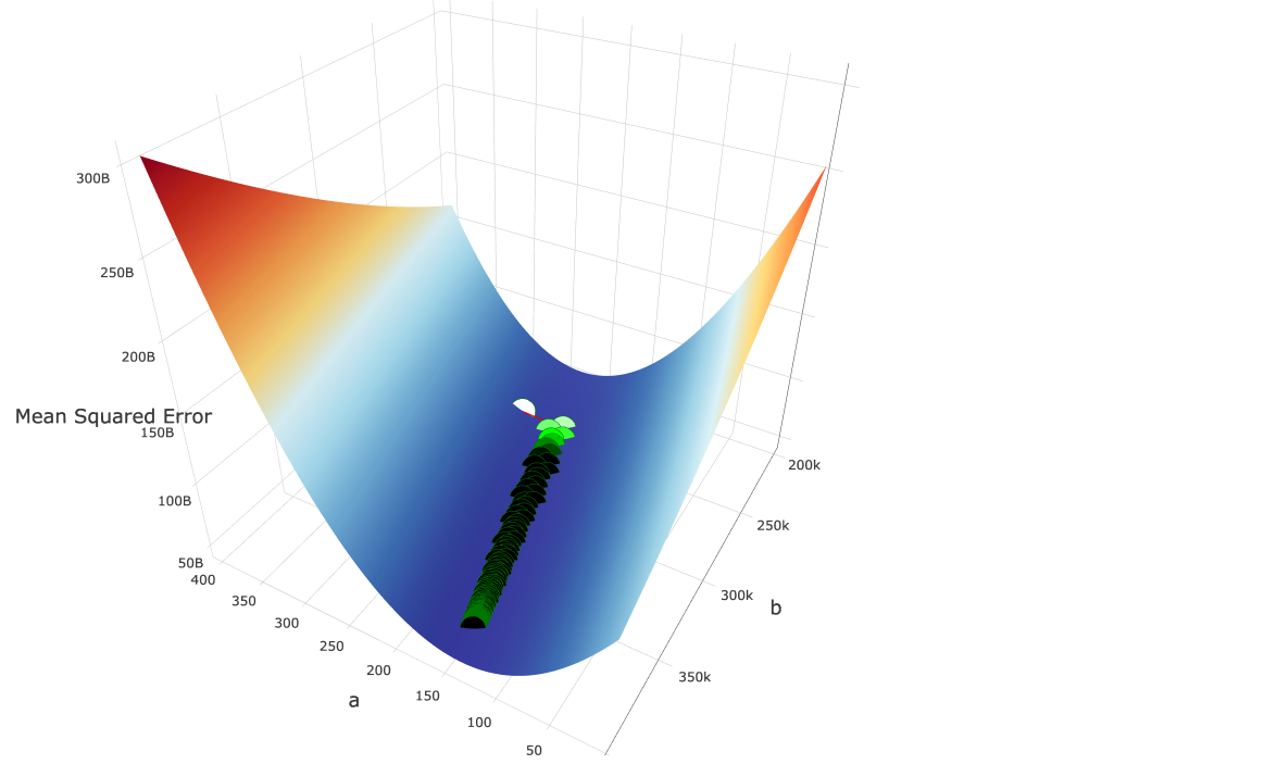
In our specific case, the above works. Our plotted gradient descent looks as follows:
In a more general, higher-dimensional example, some techniques to set learning rates such that you avoid the problems of divergence and “valley-jumping” include:
- Momentum - Add an additional term to the weight update formula, which, in our “ball down the hill” analogy, will help to get our ball rolling by compounding past gradients.
- Backtracking Line Search - Dynamically make smart choices for the learning rate at each iteration by taking a step far enough in the direction of the gradient, but not so far that we increase our error.
- Stochastic Gradient Descent - A faster (and often better) optimization algorithm that calculates gradients from single (\(x, y\)) samples, rather than the entire batch. The additional noise can be of help here, as you may get an errant data point that kicks off your path down the valley, rather than our divergent model above.
- Normalization of Data - Normalizing data creates a less elliptical contour, and will influence our objective function to have a more concentric circle countour (think a circular mountain base instead of an elliptical base!).
We will not cover these here for the brevity’s sake, but feel free to explore on your own.